


 This is the english version.
  Für die deutschsprachige Version geht es hier entlang.
Critical value for the dark energy ΩΛ in a closed universe; a smaller value leads to a Big Crunch, the exact value brings the expansion to a halt and a larger value leads to eternal accelerated expansion since then the Hubbleparameter never reaches 0 but converges to a constant value:
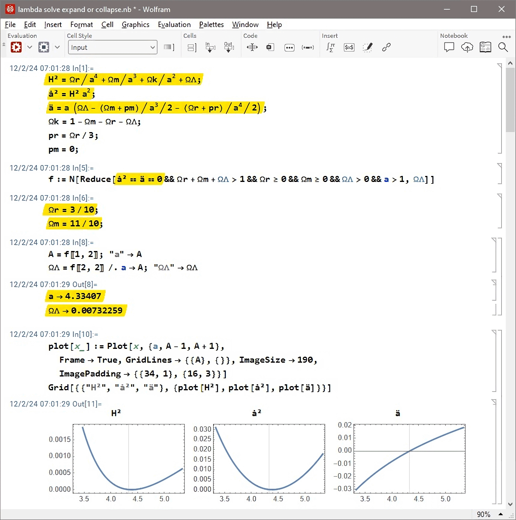
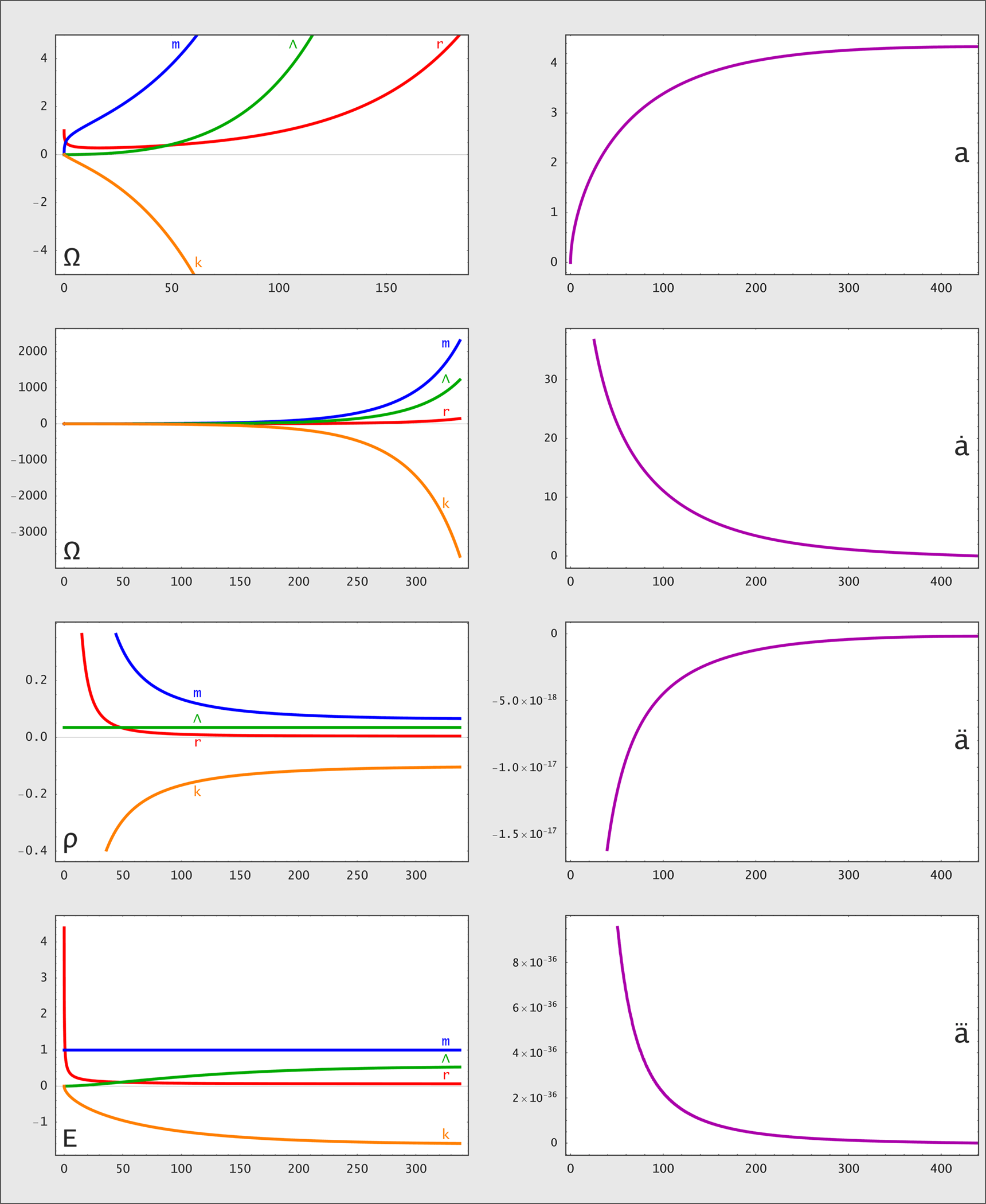
Example: at In[1] we define the normalized Hubbleparameter H and the first and second time derivatives (ȧ and ä) of the normalized scalefactor as well as the relations between pressure, density and curvature. At In[5] the velocity and acceleration of the expansion are set to 0 to solve for the limit between expansion and contraction (all the other time derivatives of a also become 0 there). At In[6] we choose our values for the matter Ωm and radiation Ωr. At In/Out[8] we evaluate the required dark energy ΩΛ and the scalefactor a when the equilibrium occurs and plot the functions at Out[11]. The plot values right of the vertical gridline belong to such values of a which are reached at no predictable time t since at the maximal value of a, here a=4.33407, we get H=0 and dH/dt=0, which is an unstable equilibrium:
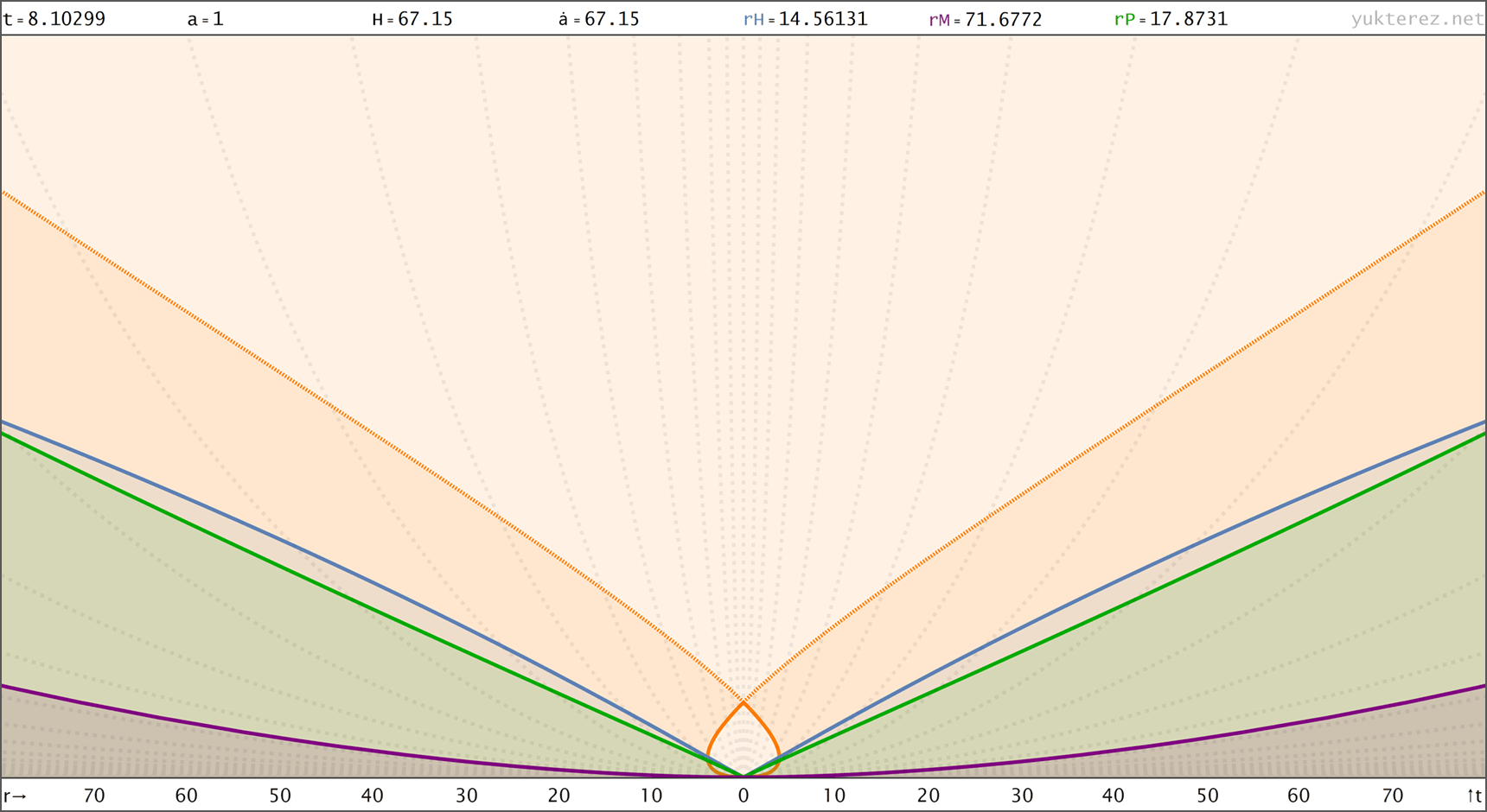
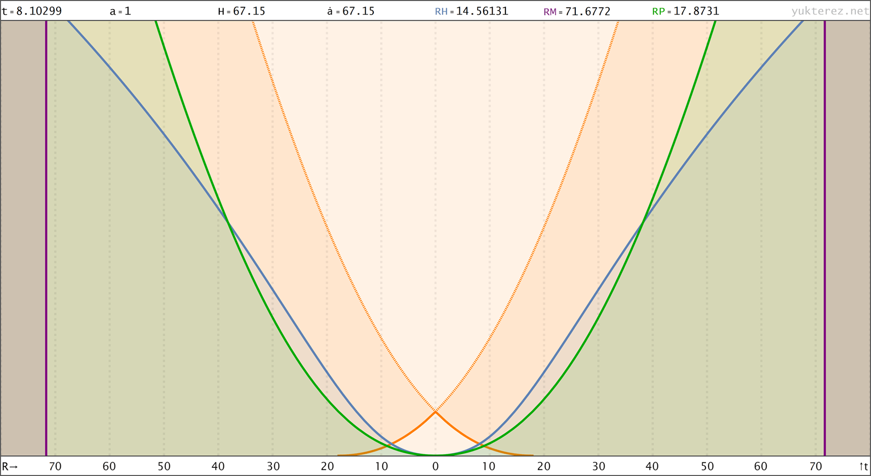
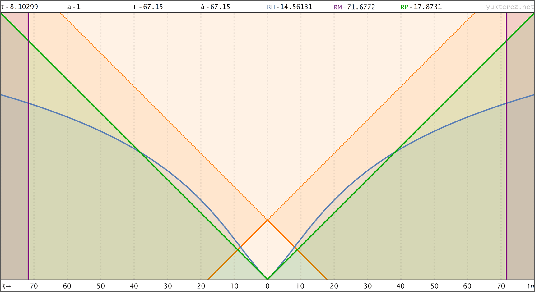
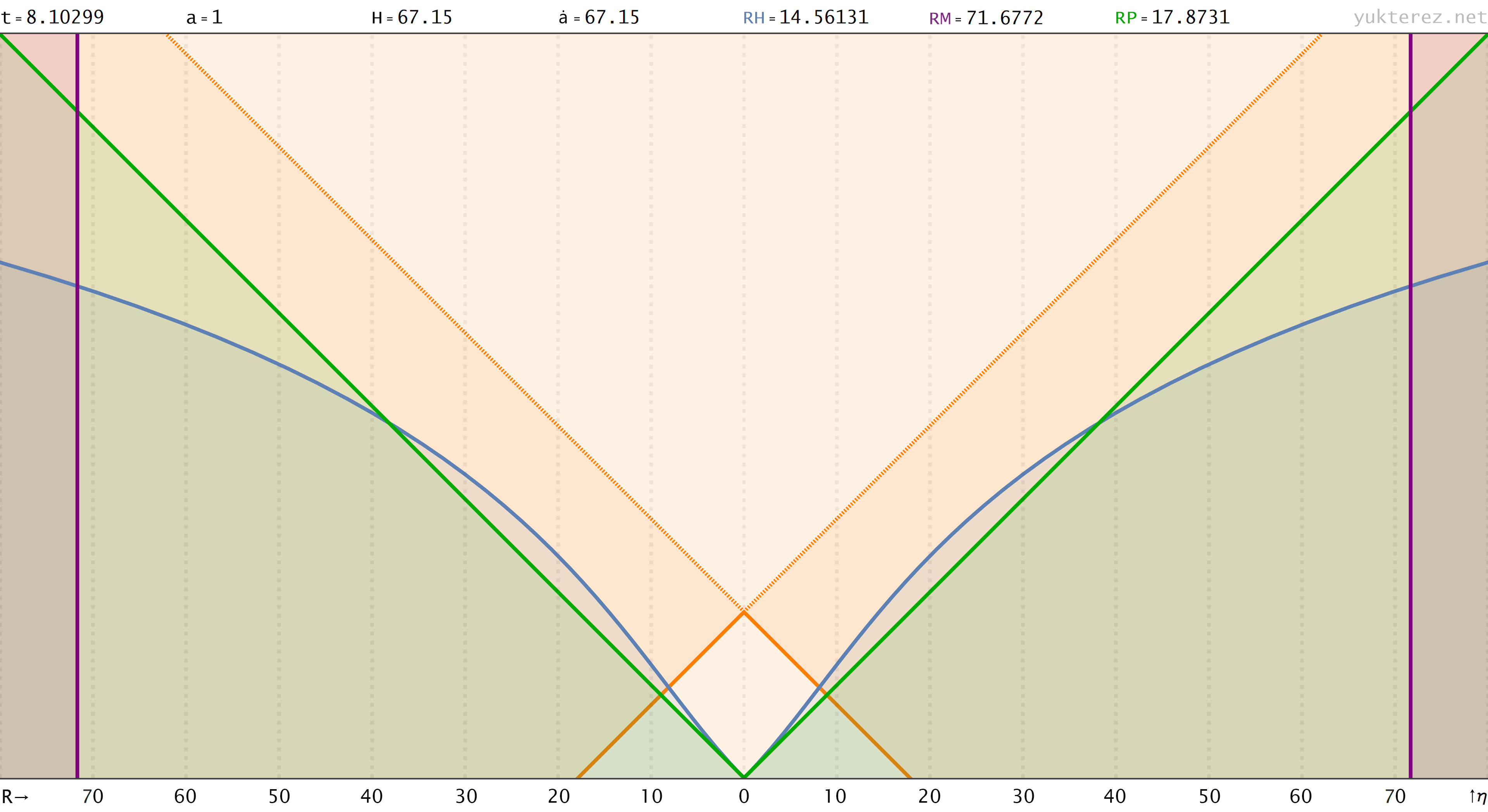
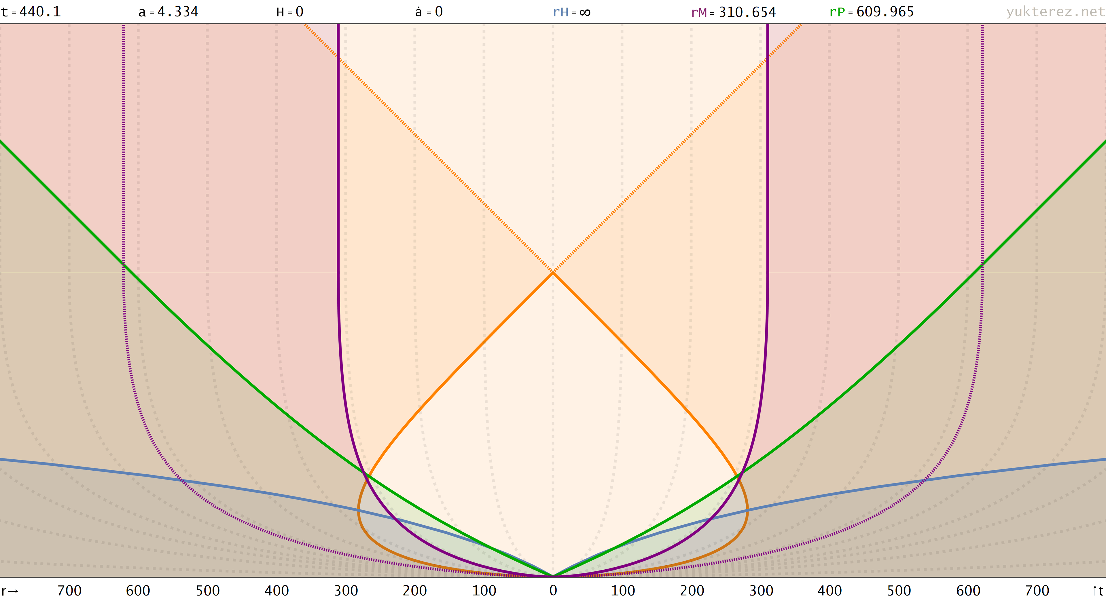
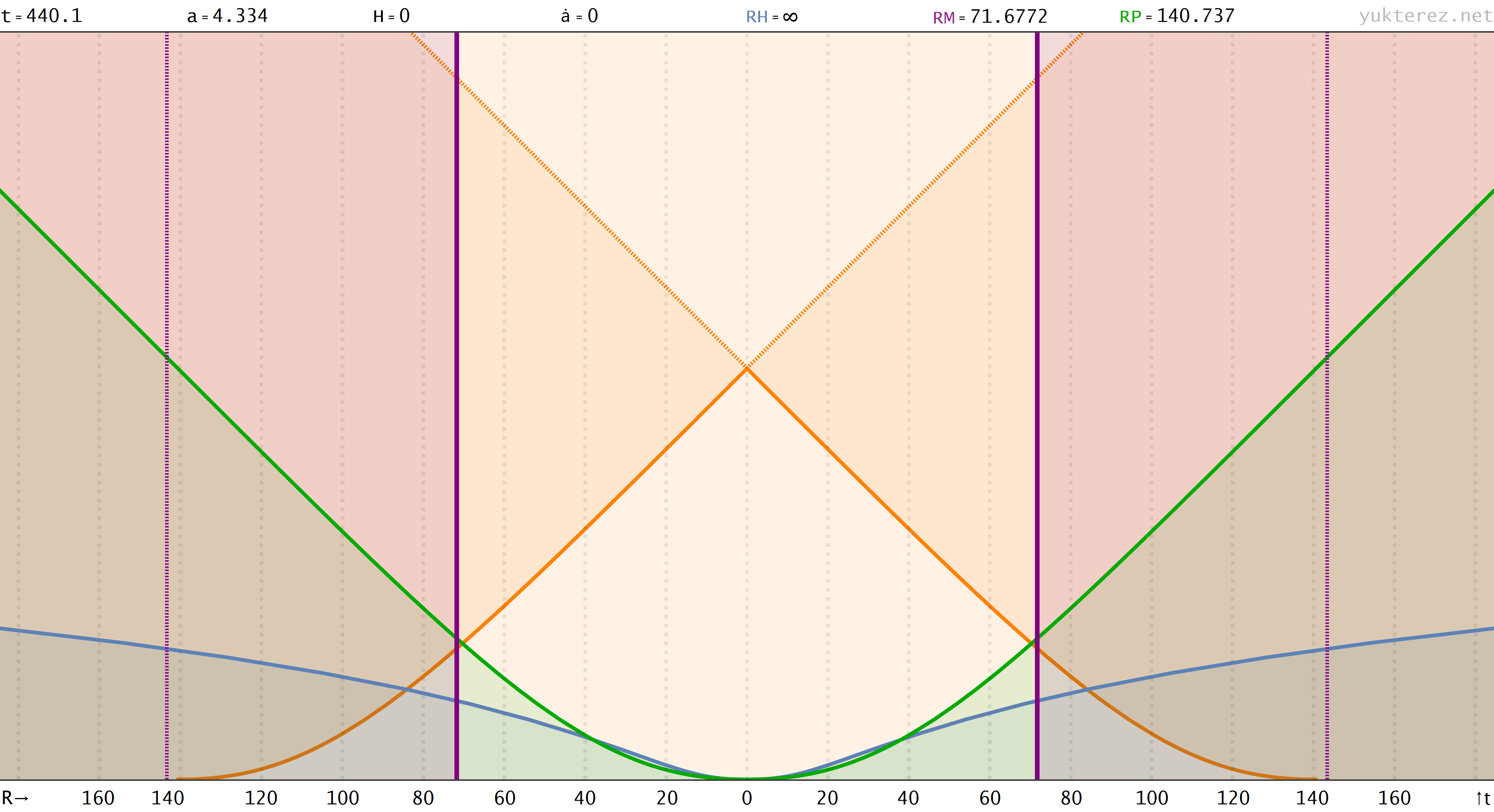
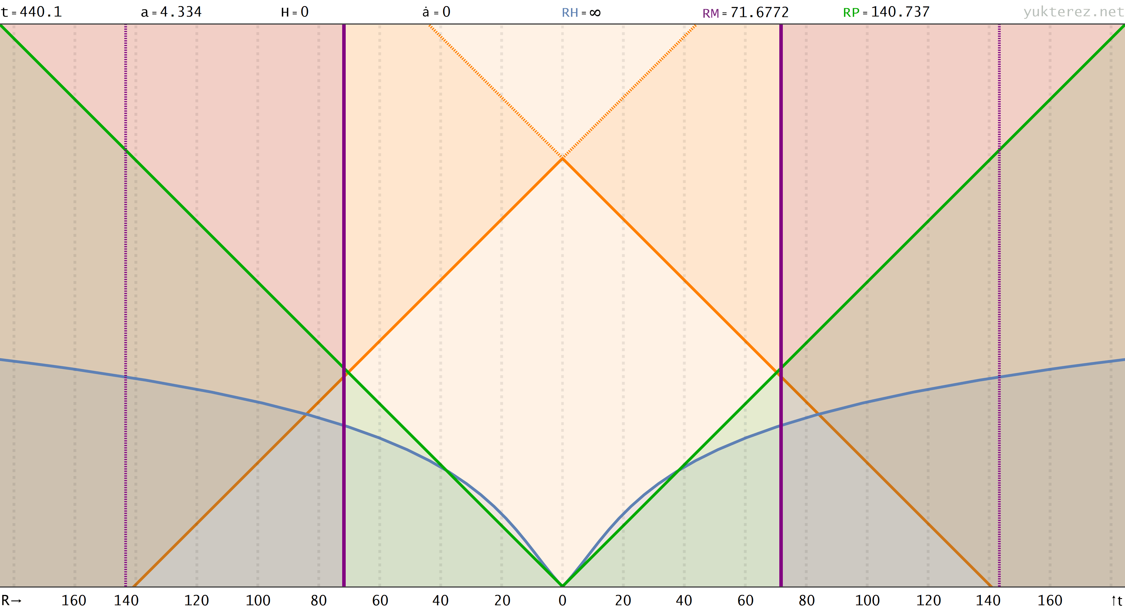
Spacetime diagrams of the universe above in proper distance r(t), comoving distance R(t) & conformal time R(η) coordinates. rH: Hubble radius (blue), rE: Event horizon (none), rP: Particle horizon (green), rM: Antipode πrK (purple), Orange curve: Past light cone, Dashed orange: Future light cone, Dashed gray: Comoving world lines, R=r/a:
For the closed FLRW metric in hyperspherical and circumferencial coordinates see here.
Code: Alles auswählen
   (* | Solver for the critical value of ΩΛ in a closed universe || yukterez.net | *)

   Ωk = 1-Ωm-Ωr-ΩΛ;
   pr = Ωr/3;
   pm = 0;
   H² = Ωr/a^4+Ωm/a^3+Ωk/a^2+ΩΛ;
   ȧ² = H² a^2;
   ä  = a (ΩΛ-(Ωm+pm)/a^3/2-(Ωr+pr)/a^4/2);

   Ωr = 3/10;
   Ωm = 11/10;

   f  = Reduce[ȧ²==ä==0 && Ωr+Ωm+ΩΛ>1 && Ωr>=0 && Ωm>=0 && ΩΛ>0 && a>1, ΩΛ]
   A  = N[f[[1,2]]]
   ΩΛ = N[f[[2,2]]]/.a->A

   plot[x_]:=Plot[x, {a, A-1, A+1}, Frame -> True, GridLines -> {{A}, {}}]
   "H²"->plot[H²]
   "ȧ²"->plot[ȧ²]
   "ä"->plot[ä]

   Quit[]
Example: at In[1] we define the normalized Hubbleparameter H and the first and second time derivatives (ȧ and ä) of the normalized scalefactor as well as the relations between pressure, density and curvature. At In[5] the velocity and acceleration of the expansion are set to 0 to solve for the limit between expansion and contraction (all the other time derivatives of a also become 0 there). At In[6] we choose our values for the matter Ωm and radiation Ωr. At In/Out[8] we evaluate the required dark energy ΩΛ and the scalefactor a when the equilibrium occurs and plot the functions at Out[11]. The plot values right of the vertical gridline belong to such values of a which are reached at no predictable time t since at the maximal value of a, here a=4.33407, we get H=0 and dH/dt=0, which is an unstable equilibrium:
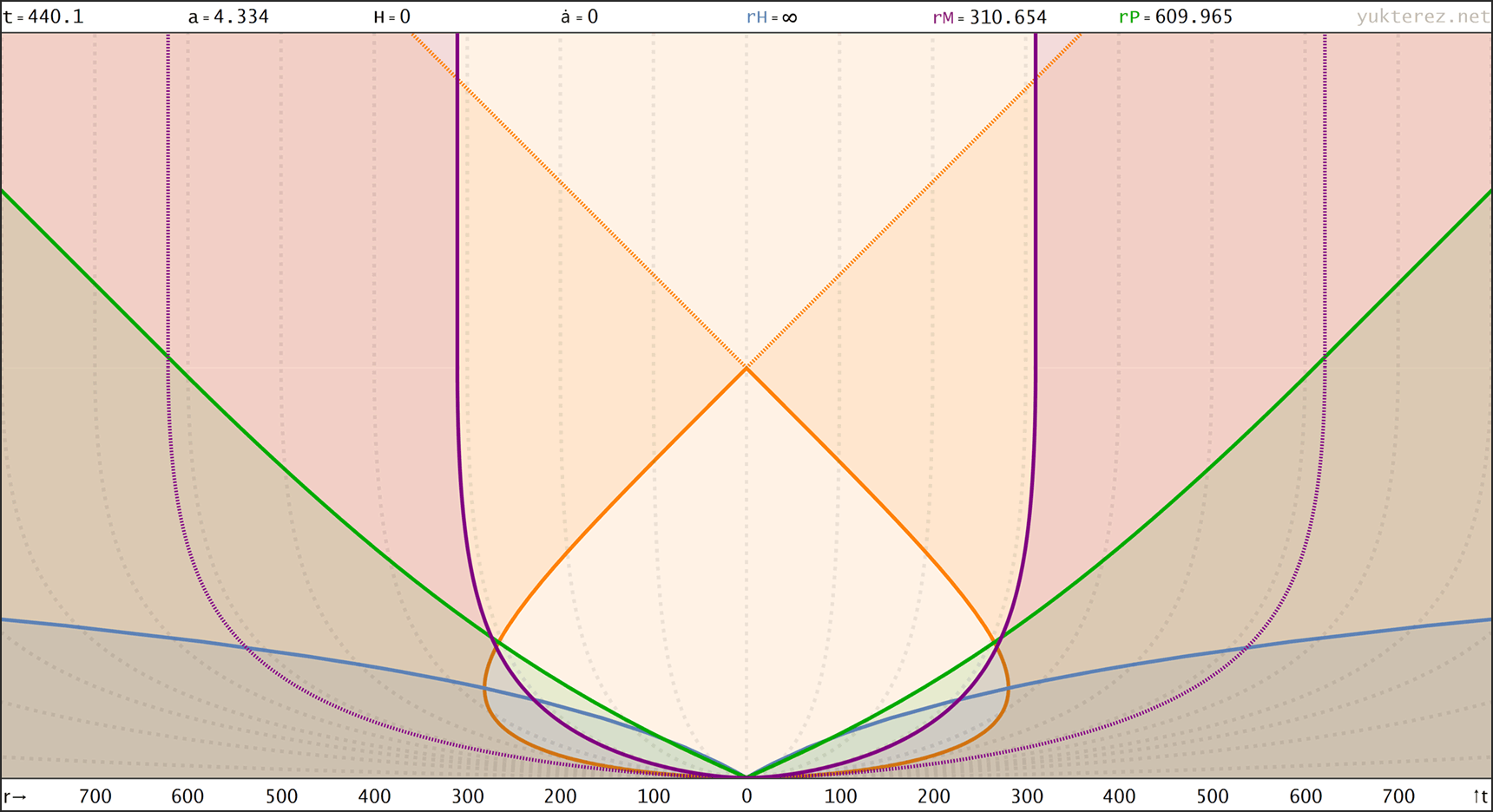
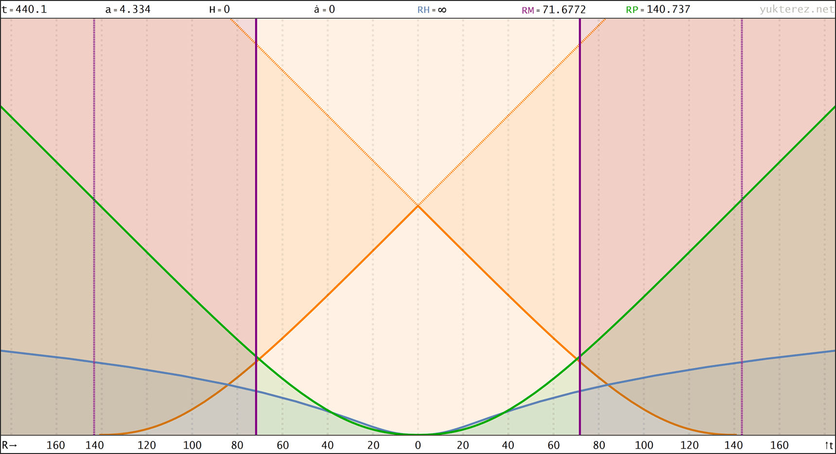
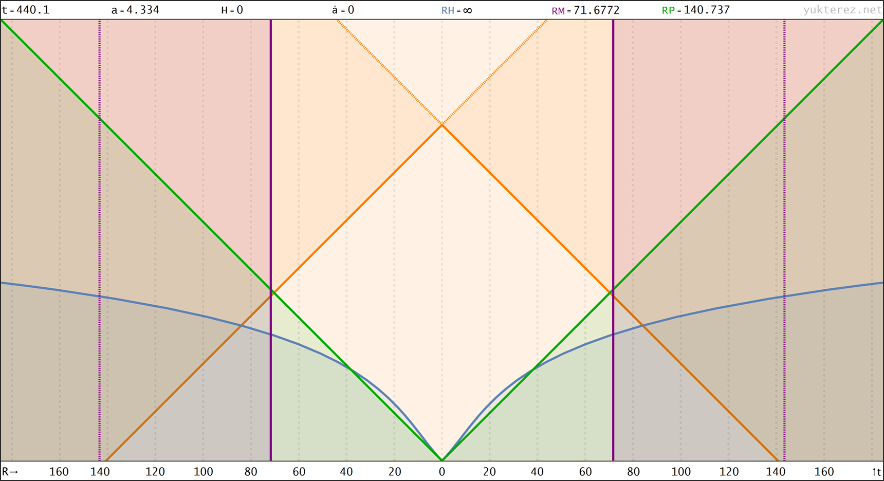
Spacetime diagrams of the universe above in proper distance r(t), comoving distance R(t) & conformal time R(η) coordinates. rH: Hubble radius (blue), rE: Event horizon (none), rP: Particle horizon (green), rM: Antipode πrK (purple), Orange curve: Past light cone, Dashed orange: Future light cone, Dashed gray: Comoving world lines, R=r/a:
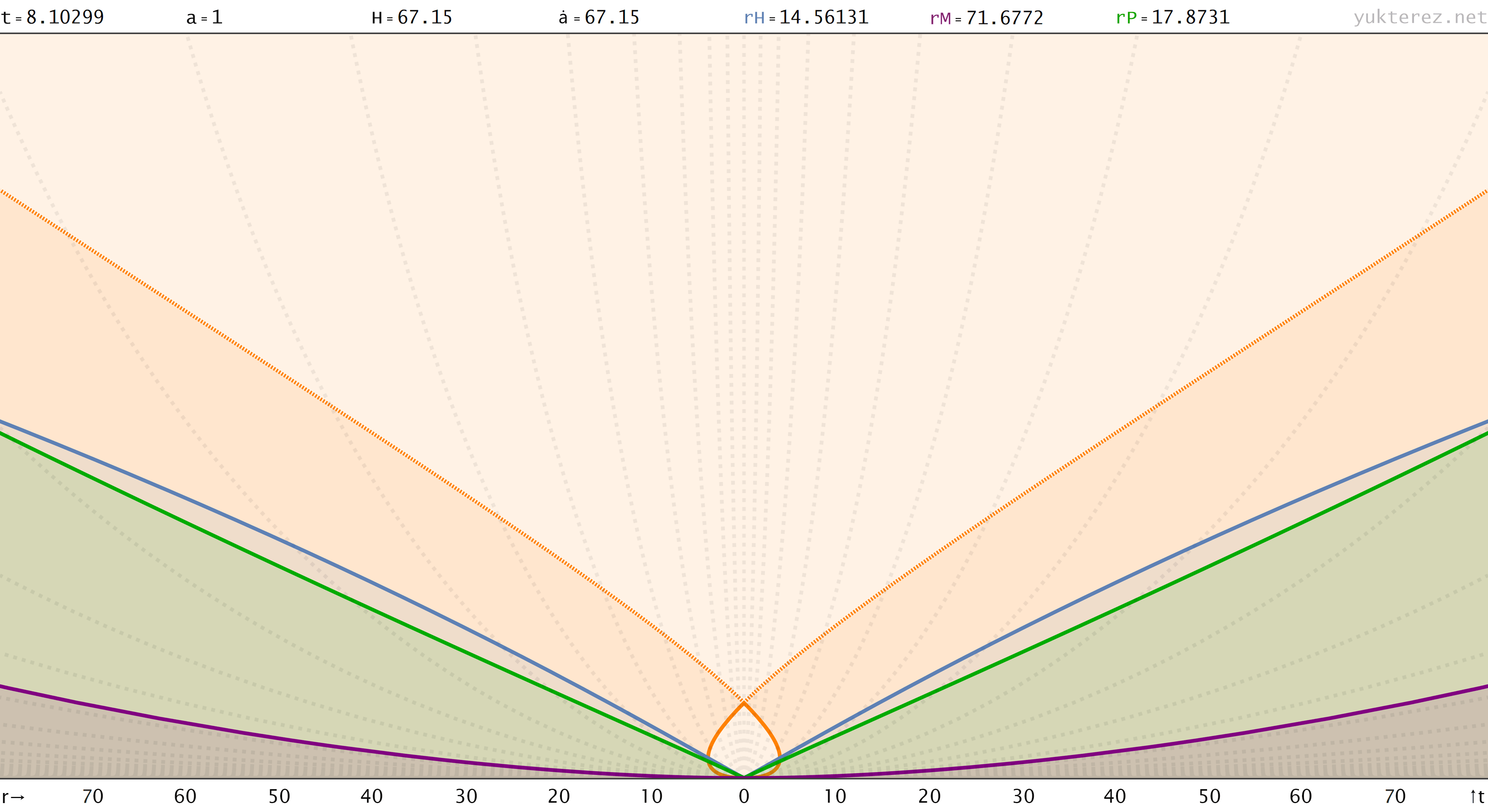
↑ proper, r(t) ◉ ↓ comoving, R(t)
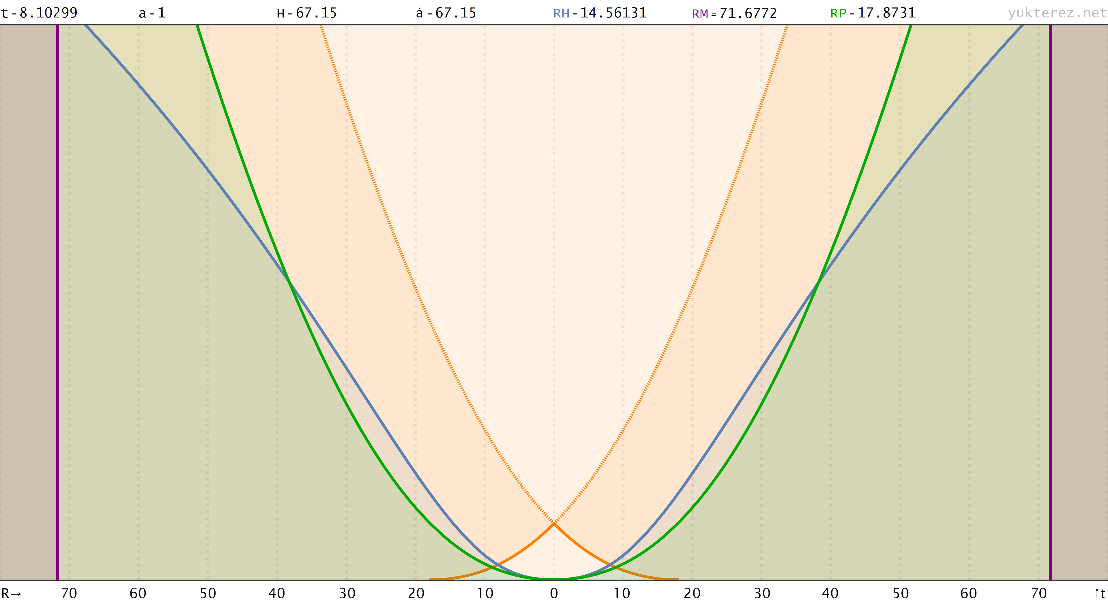
↑ comoving, R(t) ◉ ↓ conformal, R(η)
↑ t = 8.1 Gyr, a = 1 ◉ ↓ t = 440.1 Gyr, a = 4.334
↑ proper, r(t) ◉ ↓ comoving, R(t)
↑ comoving, R(t) ◉ ↓ conformal, R(η)
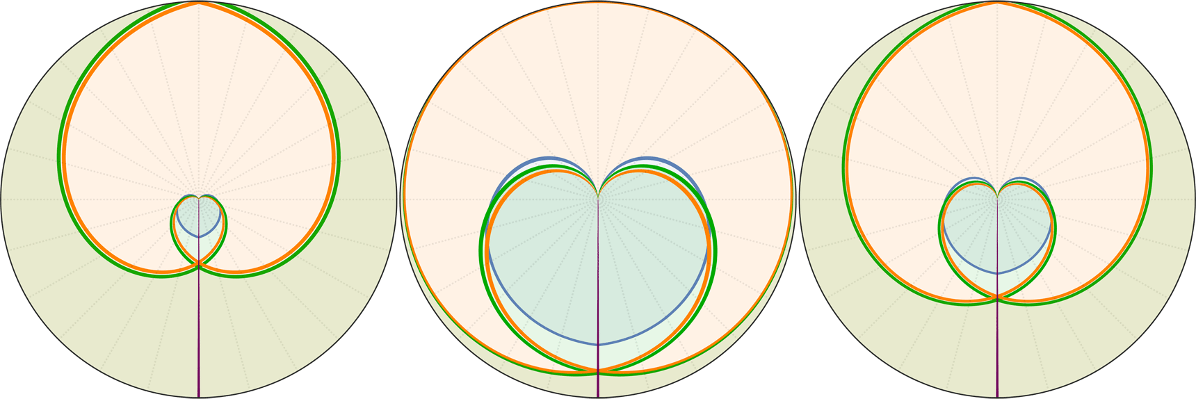
↑ conformal, R(η) ◉ ↓ polar, R(t)→φ(Я) & R(a)→φ(Я) & R(η)→φ(Я)

↑ spacetime diagrams ◉ ↓ Ω, ρ, E, a, ȧ, ä as functions of t
For the closed FLRW metric in hyperspherical and circumferencial coordinates see here.
Code: Alles auswählen
   (* | Evolution of a closed FLRW Universe that reaches an unstable equilibrium | *)

   set = {"GlobalAdaptive", "MaxErrorIncreases"->100,
   Method->"GaussKronrodRule"};                                (* Integration Rule *)
   n = 100;                                                     (* Recursion Depth *)
   int[f_, {x_, xmin_, xmax_}] :=                                      (* Integral *)
   NIntegrate[f, {x, xmin, xmax},
   Method->set, MaxRecursion->n, WorkingPrecision->wp];
   wp = MachinePrecision;                                     (* Working Precision *)
   im = 200;                                                         (* Image Size *)
   ηmax = 800; pmax = 800;                                           (* Plot Range *)
   amax = Root[4+11#-10#^2-33#^3+8#^4&, 2, 0];             (* Maximal Scale Factor *)
   tmax = 444 Gyr;                                            (* Integration Limit *)

   c = 299792458 m/sek;                                              (* Lightspeed *)
   G = 667384*^-16 m^3 kg^-1 sek^-2;                            (* Newton Constant *)
   Gyr = 10^7*36525*24*3600 sek;                                  (* Billion Years *)
   Glyr = Gyr*c;                                             (* Billion Lightyears *)
   Mpc = 30856775777948584200000 m;                                  (* Megaparsec *)
   ρc[H_] := 3H^2/8/π/G;                                       (* Critical Density *)
   ρΛ = ρc[H0] ΩΛ;                                          (* Dark Energy Density *)
   kg = m = sek = 1;                                                   (* SI Units *)

   ΩR = 3/10;                          (* Radiation Proportion including Neutrinos *)
   ΩM = 11/10;                          (* Matter Proportion including Dark Matter *)
   ΩΛ = 3/32+(77 Root[4+11#-10#^2-33#^3+8#^4&, 2, 0])/16+
   (203 Root[4+11#-10#^2-33#^3+8#^4&, 2, 0]^2)/160-
   (11 Root[4+11#-10#^2-33#^3+8#^4&, 2, 0]^3)/20;        (* Dark Energy Proportion *)
   ΩT = ΩR+ΩM+ΩΛ;                           (* Total Density over Critical Density *)
   ΩK = 1-ΩT;                                                 (* Curvature Density *)
   rK = c/H0/Sqrt[-ΩK];                                        (* Curvature Radius *)

   H0 = 67150 m/Mpc/sek;                                        (* Hubble Constant *)
   H[a_] := H0 Sqrt[ΩR/a^4+ΩM/a^3+ΩK/a^2+ΩΛ]                   (* Hubble Parameter *)

   sol = Quiet[NDSolve[{A'[t]/A[t] == H[A[t]], A[0] == 1*^-15,
   WhenEvent[Abs[A[t]] == amax, tMax=t; "StopIntegration"]},
   A, {t, 0, tmax},
   MaxSteps->∞, WorkingPrecision->wp]];

   â[t_] := Evaluate[(A[t]/.sol)[[1]]];                (* Scale Factor a by Time t *)
   a[t_] := If[t<tmax, â[t], amax]; If[t>tmax, amax, â[t]];    (* Optimized a of t *)
   т[a_] := int[1/A/H[A], {A, 0, a}];                  (* Time t by Scale Factor a *)

   rP[t_] := a[t] int[c/a[т], {т, 0, t}];          (* Proper Particle Horizon by t *)
   rp[a_] := a int[c/A^2/H[A], {A, 0, a}];         (* Proper Particle Horizon by a *)
   RP[t_] := int[c/a[т], {т, 0, t}];             (* Comoving Particle Horizon by t *)
   Rp[a_] := int[c/A^2/H[A], {A, 0, a}];         (* Comoving Particle Horizon by a *)

   rE[t_] := Nothing;                                 (* Proper Event Horizon by t *)
   re[a_] := Nothing;                                 (* Proper Event Horizon by a *)
   RE[t_] := Nothing;                               (* Comoving Event Horizon by t *)
   Rε[a_] := Nothing;                               (* Comoving Event Horizon by a *)

   rL[t0_, t_] := a[t] int[c/a[т], {т, t, t0}];          (* Proper Light Cone by t *)
   rl[a0_, a_] := a int[c/A^2/H[A], {A, a, a0}];         (* Proper Light Cone by a *)
   RL[t0_, t_] := int[c/a[т], {т, t, t0}];             (* Comoving Light Cone by t *)
   Rl[a0_, a_] := int[c/A^2/H[A], {A, a, a0}];         (* Comoving Light Cone by a *)

   rH[t_] := c/H[a[t]];                               (* Proper Hubble Radius by t *)
   rh[a_] := c/H[a];                                  (* Proper Hubble Radius by a *)
   RH[t_] := c/H[a[t]]/a[t];                        (* Comoving Hubble Radius by t *)
   Rh[a_] := c/H[a]/a;                              (* Comoving Hubble Radius by a *)

   t0 = Quiet[Re[t/.FindRoot[a[t]-1, {t, 10 Gyr}]]]; ti = t Gyr; τi = τ Gyr;
   "t0"->t0/Gyr "Gyr"                                              (* Current Time *)
   tmax = Quiet[Re[t/.FindRoot[a[t]-amax, {t, 10 Gyr}]]]; "tmax"->tmax/Gyr "Gyr"

   ηH = Quiet[Interpolation[Join[{{0, 0}},      (* Hubble Radius by Conformal Time *)
   ParallelTable[
   {Rp[amax (Sin[π a/amax/2])^3]/Glyr, Rh[amax (Sin[π a/amax/2])^3]/Glyr},
   {a, amax/2/im, amax-amax/2/im, amax/2/im}],
   {{amax, Infinity}}, {{2 amax, Infinity}}]]];
   rpN = Rp[1]/Glyr;

   "PROPER DISTANCES, f(t)"

   pt = Quiet[Plot[
   {rH[τi]/Glyr, rP[τi]/Glyr, π rK a[τi]/Glyr},
   {τ, 0, pmax}, Frame->True, AspectRatio->pmax/pmax,
   FrameTicks->None, PlotRange->{{0, pmax}, {0, pmax}},
   PlotStyle->{{Thickness[0.005]},
   {Darker[Green], Thickness[0.005]},
   {Purple, Thickness[0.005]}},
   ImageSize->im, Filling->Top,
   FillingStyle->Opacity[0.1], ImagePadding->1,
   GridLines->{{}, {}}]];

   plot1[t_] := Rasterize[Grid[{{Rotate[Quiet[Show[Plot[
   {rL[ti, τi]/Glyr, -rL[ti, τi]/Glyr},
   {τ, 0, pmax}, Frame->True, AspectRatio->1,
   FrameTicks->None, PlotRange->{{0, pmax}, {0, pmax}},
   PlotStyle->{{Orange, Thickness[0.005]},
   {{Orange, Thickness[0.005]}, Dashed}},
   ImageSize->im, Filling->Top,
   FillingStyle->Opacity[0.1], ImagePadding->1,
   GridLines->{{}, {}}], pt]], 90 Degree]}}]];

   Do[Print[plot1[t]], {t, {tmax/Gyr}}]

   plot2 = Rasterize[Grid[{{Rotate[Quiet[Plot[
   Join[{0}, Table[n a[τ Gyr]/amax,
   {n, 100, 800, 100}], {220 a[τ Gyr], 350 a[τ Gyr]}],
   {τ, 0, pmax}, Frame->True, AspectRatio->1,
   FrameTicks->None, PlotRange->{{0, pmax}, {0, pmax}},
   PlotStyle->Table[{Dashing->Large, Thickness[0.005],
   Gray}, {n, 1, 100}], ImageSize->im,
   ImagePadding->1]], 90 Degree]}}]]

   "COMOVING DISTANCES, f(t)"

   ct = Quiet[Plot[
   {RH[τi]/Glyr, RP[τi]/Glyr, π rK/Glyr},
   {τ, 0, pmax}, Frame->True, AspectRatio->1,
   FrameTicks->None, PlotRange->{{0, pmax}, {0, pmax/amax}},
   PlotStyle->{{Thickness[0.005]},
   {Darker[Green], Thickness[0.005]},
   {Purple, Thickness[0.005]}},
   ImageSize->im, Filling->Top,
   FillingStyle->Opacity[0.1], ImagePadding->1,
   GridLines->{{}, {}}]];

   plot3[t_] := Rasterize[Grid[{{Rotate[Quiet[Show[Plot[
   {RL[ti, τi]/Glyr, -RL[ti, τi]/Glyr},
   {τ, 0, pmax}, Frame->True, AspectRatio->1,
   FrameTicks->None, PlotRange->{{0, pmax}, {0, pmax/amax}},
   PlotStyle->{{Orange, Thickness[0.005]},
   {{Orange, Thickness[0.005]}, Dashed}},
   ImageSize->im, Filling->Top,
   FillingStyle->Opacity[0.1], ImagePadding->1,
   GridLines->{{}, {}}], ct]], 90 Degree]}}]];

   Do[Print[plot3[t]], {t, {tmax/Gyr}}]

   plot4 = Rasterize[Grid[{{Rotate[Quiet[Plot[
   Join[{0}, Table[n, {n, 20, pmax, 20}]],
   {τ, 0, pmax}, Frame->True, AspectRatio->1,
   FrameTicks->None, PlotRange->{{0, pmax}, {0, pmax/amax}},
   PlotStyle->Table[{Dashing->Large, Thickness[0.005],
   Gray}, {n, 1, 100}], ImageSize->im,
   ImagePadding->1]], 90 Degree]}}]]

   "CONFORMAL DIAGRAM, f(η)"

   cη = Quiet[Plot[
   {ηH[Ct], Ct, π rK/Glyr},
   {Ct, 0, ηmax/amax}, Frame->True, AspectRatio->1,
   FrameTicks->None, PlotRange->{{0, ηmax/amax}, {0, pmax/amax}},
   PlotStyle->{{Thickness[0.005]},
   {Darker[Green], Thickness[0.005]},
   {Purple, Thickness[0.005]}},
   ImageSize->im, Filling->Top,
   FillingStyle->Opacity[0.1], ImagePadding->1,
   GridLines->{{}, {}}]];

   plot9[η_] := Rasterize[Grid[{{Rotate[Quiet[Show[Plot[
   {η-Ct, Ct-η}, {Ct, 0, ηmax/amax},
   Frame->True, AspectRatio->1,
   FrameTicks->None, PlotRange->{{0, ηmax/amax}, {0, pmax/amax}},
   PlotStyle->{{Orange, Thickness[0.005]},
   {{Orange, Thickness[0.005]}, Dashed}},
   ImageSize->im, Filling->Top,
   FillingStyle->Opacity[0.1], ImagePadding->1,
   GridLines->{{}, {}}], cη]], 90 Degree]}}]];

   Do[Print[plot9[η]], {η, {RP[tmax]/Glyr}}]

   plot10 = Rasterize[Grid[{{Rotate[Quiet[Plot[
   Join[{0}, Table[n, {n, 20, pmax, 20}]],
   {Ct, 0, ηmax}, Frame->True, AspectRatio->1,
   FrameTicks->None, PlotRange->{{0, ηmax/amax}, {0, pmax/amax}},
   PlotStyle->Table[{Dashing->Large, Thickness[0.005],
   Gray}, {n, 1, 100}], ImageSize->im,
   ImagePadding->1]], 90 Degree]}}]]

   s[text_] := Style[text, FontFamily->"Lucida Console", FontSize->36]